Visual TreeCmp: Comparison of Phylogenetic Trees on the Web

Introduction

The TreeCmp application was designed to compute distances between arbitrary (not necessary binary) phylogenetic trees. Offers an implementation of metrics allowing to compare trees with a large number of leaves.

Comparison modes

In the first step, select one of the four available comparison modes (Overlaping Pair, Window, Matrix - default, Reference trees to all input trees) as shown in Fig 1. In the case of Window mode you have to enter it's width in the additional field as shown in Fig 2.

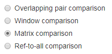
Fig. 1

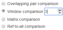
Fig. 2

In each of those available modes, different trees are compared:

overlapping pair comparison mode; every two neighboring trees from the input are compared.
window comparison mode; every two trees within a window with a specified size are compared – the average distance and the standard deviation can be computed if Include summary options is checked,
matrix comparison mode; every two trees from the input are compared.
reference trees to all input trees mode; each tree from the input is compared to all reference tree (or trees).

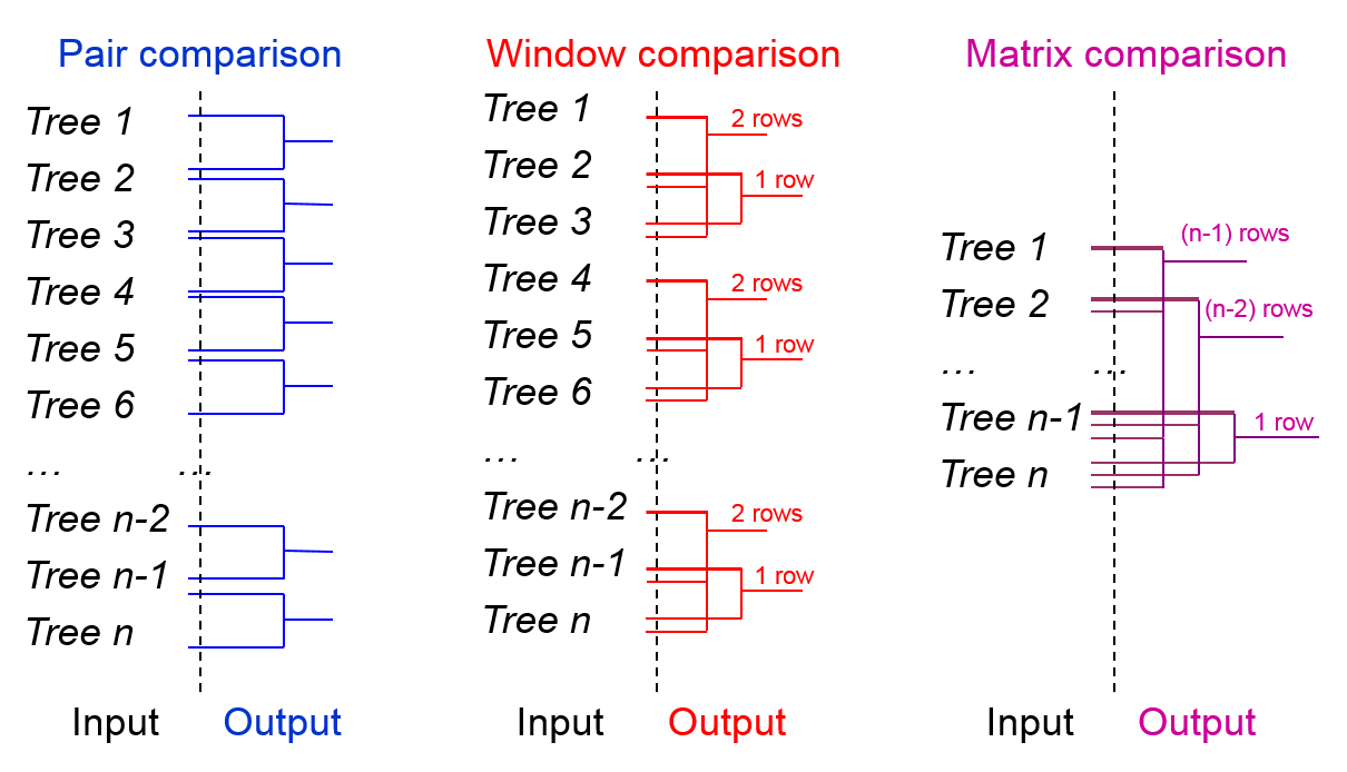
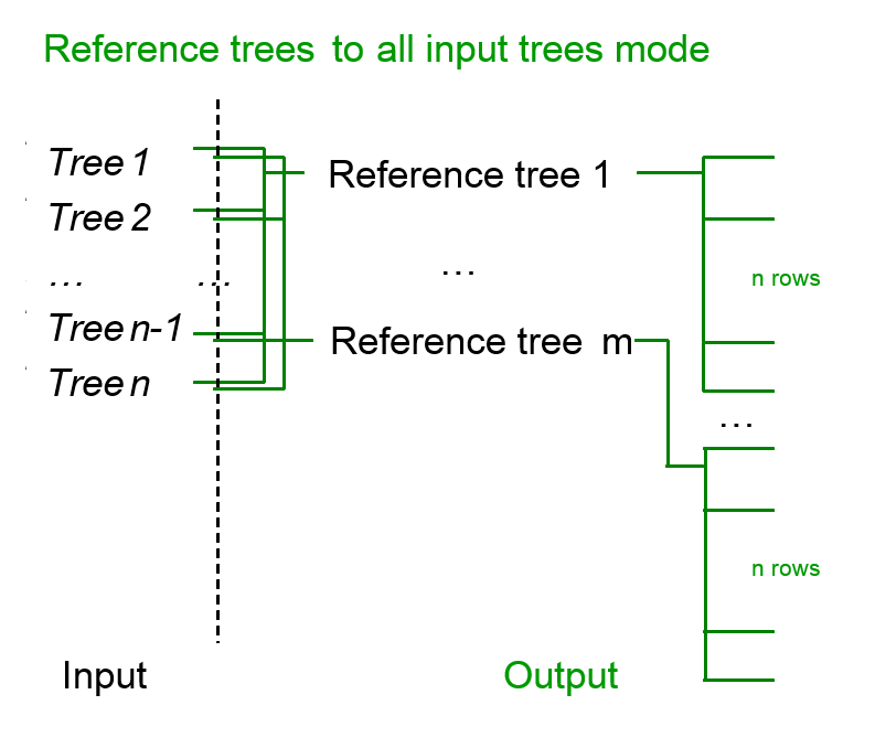
Details of the computation flow in each of these case are explained in in Fig. 3.

Fig. 3

Compared trees

The TreeCmp software was designed to support Nexus tree specifications date files (BEAST and MrBayes), where phylogenetic trees are stored in the Newick format. Note that plain text files containing only trees in this format are supported as well.
In next step compared trees should be entered, it can be done it in few ways as shown in Fig 4, You can:

enter manually or paste from the clipboard one or more phylogenetic trees separated by a semicolon to the main newick trees window (Fig. 4A).
click the button with the file icon (Fig. 4B) and then in the newly opened explorator window, select the appropriate newick file. If the file is properly loaded, its contents should be displayed in the main newick trees window and its name will be displayed in the textbox (Fig. 4C).
drag and drop file with trees on the main newick trees window, the result should be the same as in the previous case.
if you don't have any Nexus trees files, simply enter a example trees by clicking the Example Trees link (Fig. 4D). Loaded trees should be displayed in the main newick trees window main newick trees window.

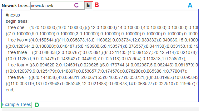
Fig. 4

Metrics

In the next step, select at least one of available phylogenetic metrics. It can be for rooted or unrooted trees, and if you are interested in more than one, you can select a few metrics as shown in Fig 5. In a special case, you can even select all.

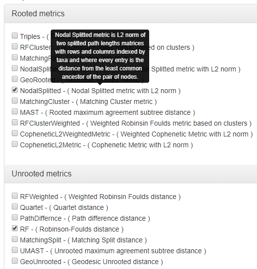
Fig. 5

Other options

Additional options are available (Fig 6):

Report normalized distances δm for a particular metric m (Bogdanowicz et al. 2012; based on an average value from pre-computed data). This functionality is available for trees with number of leaves between 4 and 1000. Note that normalized tree similarity for a particular metric m (NTSm) can be expressed by normalized distance as follows: NTSm. = 1 - δm (Bogdanowicz et al. 2012).
Prune compared trees if needed. This option is design to allow comparing trees having different (partially overlapping) sets of taxa. After using this option three additional columns appear in the output file (see section 4 for details).
Include summary section in the output file.
Zero weights allowed during using weighted metrics. If there is no weight assigned to the edge, its default value will be set to zero.
Allow only bifurcating trees.

In the last step, click Compute button to generate report (Fig 6).

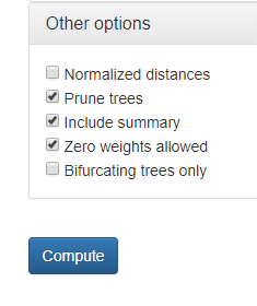
Fig. 6

Report

After completing calculations, results appear in the new tab as shown in Fig. 7. Each row (excluding header) contains information about calculated metrics for one pair of compared trees. In the first three rows we find the ordinal number and numbers of compared trees.(Fig. 7A). In subsequent columns, we can find the metrics selected in the previous step (Fig. 7B).

Each pair of compared trees can be drawn by clicking corresponding row. The visualized trees will be displayed in a new pop-up window using the Phylo.io application. Detailed information related to manipulation of displayed trees are placed in the manual available in the newly displayed window.

After using Normalized distances option the following two columns (Fig. 7C) per each chosen metric appear additionally in the output file. These columns contain the value of the distance in a particular metric divided by its empirical average value. If the number of common leaves in compared trees is out of supported range (which is form 4 to 1000), then “N/A” value is inserted. For details regarding generating phylogenetic trees under the Yule and uniform models see (McKenzie and Steel 2000; Semple and Steel 2003).

By default, data is sorted in ascending order by first column containing the ordinal numbers. We can easily change it by clicking the appropriate column header (this also applies to the order: decreasing, increasing). In order to search/filter only rows that containing a certain phrase, we can use the search control (Fig. 7D).

The displayed data (excluding filtered ones) can be easily copied to the system clipboard, saved in one of the following formats: CSV, EXCEL, PDF or printed using the appropriate button (Fig. 7E).

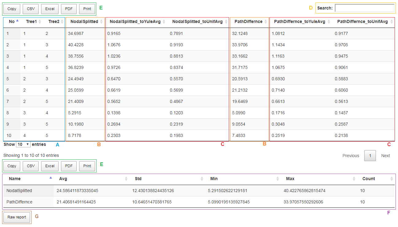
Fig. 7

The following table contains a mapping between available metrics and column names in the Report that are related to them.

Metric name in the output file	Full metric name
MatchingSplit	Matching Split distance
RF	Robinson-Foulds distance
PathDiffernce	Path difference distance
Quartet	Quartet distance
UMAST	Unrooted maximum agreement subtree distance
RFWeighted	Weighted Robinsin Foulds distance
GeoUnrooted	Geodesic Unrooted distance
MatchingCluster	Matching Cluster metric
RF_Cluster	Robinson-Foulds metric based on clusters
NodalSplitted	Nodal Splitted metric with L² norm
Triples	Triples metric
MatchingPair	Matching Pair metric
MAST	Rooted maximum agreement subtree metric
CopheneticL2Metric	Cophenetic Metric with L² norm
RFClusterWeighted	Weighted Robinson-Foulds metric based on clusters
NodalSplittedWeighted	Weighted Nodal Splitted metric with L² norm
GeoRooted	Geodesic Rooted metric
CopheneticL2WeightedMetric	Weighted Cophenetic Metric with L² norm

Using Summary option adds an additional section to the report with the following format (Fig. 7F):

Name	Avg	Std	Min	Max	Count
Metric name 1	Average value	Standard deviation value	Minimal value	Maximal value	Number of analyzed values
Metric name 2	…	…	…	…	…
…	…	…	…	…	…
Metric name n	…	…	…	…	…

After using switch Prune trees option the following three columns appear additionally in report (not used in our example).

Tree1_taxa	Tree2_taxa (or RefTree_taxa)	Common_taxa
Number of taxa in the first tree	Number of taxa in the second (or reference) tree	Number of taxa in common

Report file

By clicking the Raw report button (Fig. 7G), you can save the report in text format file . This file is tab separated text files (TSV), which means that they can be easily read by various data analysis software (e.g. MS Excel, R, OpenOffice.org). An report file consists of two sections (Fig 8). The first section contains formatted in rows values of distances in selected metrics. The second (optional) section contains summary data computed based on all rows that appears in the first section.

Fig. 8

Examples

Comparing trees using Matching Split distance

Select Window comparison and set window width to 2 as shown in Fig 9a.

Fig. 9a

Enter the following NEXUS file format content (File. 1) to the main newick trees window (Fig. 9b). This is the first way to enter compared trees described in Compared trees section.

File. 1 (testBSP.newick)

Fig. 9b

Choose Matching Split distance from available unrooted metrics (Fig. 9c) and Include summary option from Other options (Fig. 9d).

Fig. 9c

Fig. 9d

As a result (Fig. 9e), we obtain 5 comparisons and its summary.

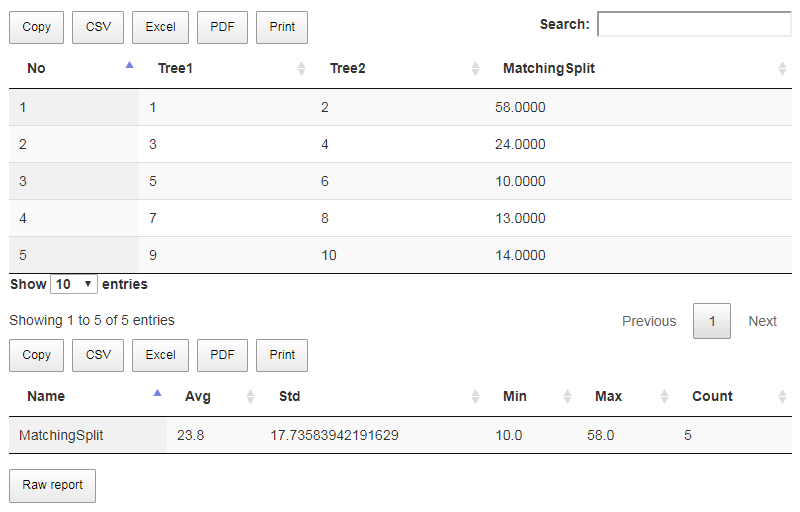
Fig. 9e

These calculations can be saved to report.txt file (Fig. 9f) by clicking the Save report button.

Fig. 9f

Computing normalized distances

Reporting distances divided by pre-computed empirical average values for random trees (generated according to Yule and uniform models, Normalized distances option) can help in an interpretation of the similarity level of analyzed trees in chosen metric. In the following example, the distance in the MS metric of each tree from a given set (File. 2) to the reference tree (File. 3) is computed. Analyzed trees have 15 leaves.

File. 2 (test_set.trees)

File. 3 (testBSP.newick)

Select Ref-to-all comparison and enter trees from a given set (File. 2) and reference tree (File. 3) to the main newick trees window as shown in Fig 10a.

Fig. 10a

Choose Matching Split distance from available unrooted metrics and Normalized distances option from Other options as shown in Fig 10b.

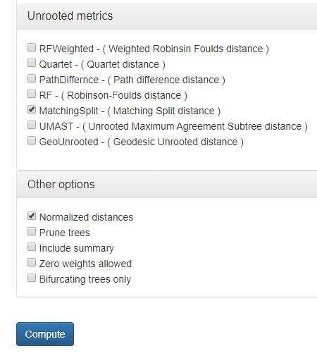
Fig. 10b

As a result (Fig. 10c), we obtain 12 comparisons without summary.

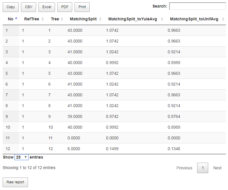
Fig. 10c

Basic interpretation of result.txt file (Fig. 10d):

Tree number 11 has the same topology as the reference tree.
Tree number 12 is very similar to the reference tree in comparison to similarly of random on 15 leaves (the normalized distance is about 0.15 and 0.13 depending on the random model).
Trees with numbers 1 to 10 are approximately as similar to the reference tree as random trees to each other (the normalized distance is close to 1).

In ordered to perform more advance similarity analysis, e.g. involving different model of generation of random trees, user my need to use TreeCmp twice:

to compute distances between custom set of random trees generated by other software, e.g. Evolver application form PAML package (http://abacus.gene.ucl.ac.uk/software/paml.html) to obtain the empirical average distance in a particular metric or its distribution,
to compute the distance between analyzed trees.

Fig. 10d

Finding the most similar trees in the input file

The most convenient comparison mode for such purpose is a Matrix (default) mode. In the following example (File. 4), the Matching Split distance is used.

File. 4 (plain2.trees)

Trees number 2, i.e.: (a,b,(c,(d,e))) and 3, i.e.:(((a,b),c),d,e) in the input are the most similar. In fact, they have the same topology (trees are assumed to be unrooted as metric for unrooted trees is used) because their distance is 0 as shown in Fig. 11 (report.txt file).

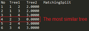
Fig. 11

Exporting data to other applications: MS Excel, R

The report can be easily copied to clipboard, saved in one of three formats: MsExcel, CSV or PDF or printed, see Fig. 12.

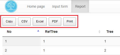
Fig. 12

In order to pass data to R (http://www.r-project.org/) it is convenient to have the TreeCmp result file in a simple tabular form (therefore, it is recommended to avoid Include summary option, because it results in generation the summary section, which disturb the tabular order). Such files can be easily read by R environment by using for example the read.table function as follows:
treeCmpData<-read.table("C:\\Program Files\\TreeCmp\\examples\\plain\\result.txt", header = TRUE, sep = "\t")
In the example, the file to read “result.txt” is placed in “C:\Program Files\TreeCmp\examples\plain” folder.